# 1.Overview
Supervise training(give the right answer first-training set examples) Unsupervise training Asymptotes Superscript
Regression problem Classification problem
# 2.Linear regression
最小二乘法(least squares method) https://www.youtube.com/watch?v=MC7l96tW8V8 最小二乘法(Least Square)和最大似然估计 Least squares cost function 最小二乘法的本质是什么? https://www.zhihu.com/question/37031188 在进行线性回归时,为什么最小二乘法是最优方法 https://www.zhihu.com/question/24095027
什么时候最小二乘参数估计和最大似然估计结果相同? https://www.jiqizhixin.com/articles/2018-01-09-6 最小二乘法是另一种常用的机器学习模型参数估计方法。结果表明,当模型向上述例子中一样被假设为高斯分布时,MLE 的估计等价于最小二乘法。 直觉上,我们可以通过理解两种方法的目的来解释这两种方法之间的联系。对于最小二乘参数估计,我们想要找到最小化数据点和回归线之间距离平方之和的直线(见下图)。在最大似然估计中,我们想要最大化数据同时出现的总概率。当待求分布被假设为高斯分布时,最大概率会在数据点接近平均值时找到。由于高斯分布是对称的,这等价于最小化数据点与平均值之间的距离。
# 2.1 Univariate linear regression / Linear regression with one variable
两种方法求系数
1.直接数学技巧
∑y = na + b∑x
∑xy = ∑xa + b∑x²
=>
b = n∑xy – (∑x)(∑y) n∑x² – (∑x)²
a = ∑y – b∑x n
https://www.accountingverse.com/managerial-accounting/cost-behavior/least-squares-method.html
变形/形式变换 https://blog.csdn.net/u011026329/article/details/79183114
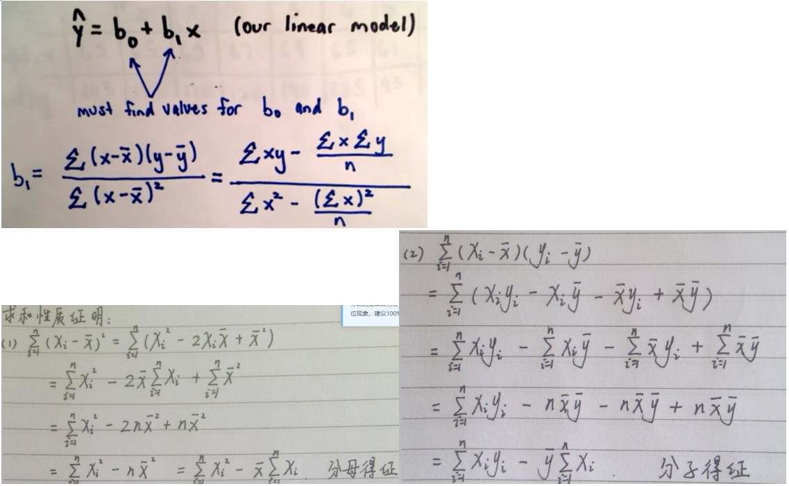
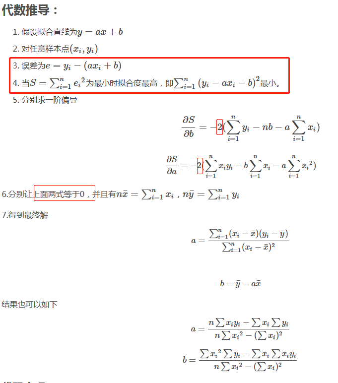
2.最小二乘法求导
# 2.2 Linear regression with multiple variable
因为系数过多无法像上面直接求解,另外如果直接求解无法继续用regularlization来惩罚系数从而控制overfitting,所以直接根据最小二乘法构造cost function

http://www.fanyeong.com/2017/03/29/machine-learning-%E7%BA%BF%E6%80%A7%E5%9B%9E%E5%BD%92%EF%BC%88linear-regression%EF%BC%89/
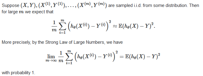
上面图中提到的除m更好是用大数定理中心极限定理来解释,即当样本足够大,均值等于数学期望(算术平均值),此处即误差的均值等于数学期望
 https://stats.stackexchange.com/questions/155580/cost-function-in-ols-linear-regression
Gradient Descent, Step-by-Step https://www.youtube.com/watch?v=sDv4f4s2SB8
梯度下降与最小二乘法的区别 https://blog.csdn.net/hu_666666/article/details/127204192
梯度下降
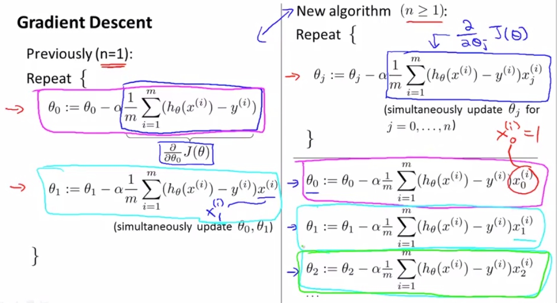
为什么梯度是函数下降最快的方向,推导 (opens new window) 推导关键词:全微分 点乘 (opens new window)
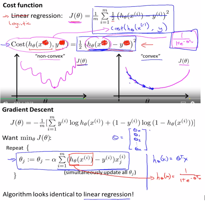
# 3. Logistic regression
- 线性回归要求变量服从正态分布,logistic回归对变量分布没有要求。
- 线性回归要求因变量是连续性数值变量,而logistic回归要求因变量是分类型变量。
- 线性回归要求自变量和因变量呈线性关系,而logistic回归不要求自变量和因变量呈线性关系
- logistic回归是分析因变量取某个值的概率与自变量的关系,而线性回归是直接分析因变量与自变量的关系
- 线性回归是拟合函数,逻辑回归是预测函数
- 线性回归的参数计算方法是最小二乘法,逻辑回归的参数计算方法是梯度下降
Sigmoid function / logistic function 为什么采用sigmoid function(正态分布)作为cost function 跟 最大似然估计有关 http://www.hanlongfei.com/%E6%9C%BA%E5%99%A8%E5%AD%A6%E4%B9%A0/2015/08/05/mle/
regularization
# 神经网络
交互式图解人工智能 (AI) 手写数字识别 (opens new window)
数字识别例子 Neural Networks Explained from Scratch using Python (opens new window)
特征=>卷积核 激活函数=>不能用阶跃函数 梯度下降=>反向传播
神经网络=>全连接 卷积神经网络=>卷积方式连接 transformer神经网络架构=>transformer连接方式
CNN: 一图胜千言:没有数学推导,5分钟理解CNN(卷积神经网络)的实现过程 https://mp.weixin.qq.com/s/AjnS2ljdtfAkQ9PGHYbOZQ https://medium.com/impactai/cnns-from-different-viewpoints-fab7f52d159c
# Quiz
Linear Regression with One Variable
Consider the problem of predicting how well a student does in her second year of college/university, given how well she did in her first year. Specifically, let x be equal to the number of "A" grades (including A-. A and A+ grades) that a student receives in their first year of college (freshmen year). We would like to predict the value of y, which we define as the number of "A" grades they get in their second year (sophomore year). Here each row is one training example. Recall that in linear regression, our hypothesis is hθ(x)=θ0+θ1x, and we use m to denote the number of training examples. | x | y | |---|---| | 5 | 4 | | 3 | 4 | | 0 | 1 | | 4 | 3 | For the training set given above (note that this training set may also be referenced in other questions in this quiz), what is the value of m? In the box below, please enter your answer (which should be a number between 0 and 10).
For this question, assume that we are using the training set from Q1. Recall our definition of the cost function was J(θ0,θ1)=12m∑mi=1(hθ(x(i))−y(i))2. What is J(0,1)? In the box below, please enter your answer (Simplify fractions to decimals when entering answer, and '.' as the decimal delimiter e.g., 1.5).
Suppose we set θ0=−1,θ1=2 in the linear regression hypothesis from Q1. What is hθ(6)?
Let f be some function so that f(θ0,θ1) outputs a number. For this problem, f is some arbitrary/unknown smooth function (not necessarily the cost function of linear regression, so f may have local optima). Suppose we use gradient descent to try to minimize f(θ0,θ1) as a function of θ0 and θ1. Which of the following statements are true? (Check all that apply.) If θ0 and θ1 are initialized so that θ0=θ1, then by symmetry (because we do simultaneous updates to the two parameters), after one iteration of gradient descent, we will still have θ0=θ1. If the learning rate is too small, then gradient descent may take a very long time to converge. If θ0 and θ1 are initialized at a local minimum, then one iteration will not change their values. Even if the learning rate α is very large, every iteration of gradient descent will decrease the value of f(θ0,θ1).
Suppose that for some linear regression problem (say, predicting housing prices as in the lecture), we have some training set, and for our training set we managed to find some θ0, θ1 such that J(θ0,θ1)=0. Which of the statements below must then be true? (Check all that apply.) Our training set can be fit perfectly by a straight line, i.e., all of our training examples lie perfectly on some straight line. For this to be true, we must have y(i)=0 for every value of i=1,2,…,m. For this to be true, we must have θ0=0 and θ1=0 so that hθ(x)=0 Gradient descent is likely to get stuck at a local minimum and fail to find the global minimum.
Many substances that can burn (such as gasoline and alcohol) have a chemical structure based on carbon atoms; for this reason they are called hydrocarbons. A chemist wants to understand how the number of carbon atoms in a molecule affects how much energy is released when that molecule combusts (meaning that it is burned). The chemist obtains the dataset below. In the column on the right, “kJ/mol” is the unit measuring the amount of energy released. | Name of molecule | Number of hydrocarbons in molecule(x) | Heat release when burned(kJ/mol)(y)| |---|---|---| | methane | 1 | -890 | | ethene | 2 | -1411 | | ethane | 2 | -1560 | | propane | 3 | -2220 | | cyclopropane | 3 | -2091 | | butane | 4 | -2878 | | pentane | 5 | -3537 | | benzene | 6 | -3268 | | cycloexane | 6 | -3920 | | hexane | 6 | -4163 | | octane | 8 | -5471 | | napthalene | 10 | -5157 |
You would like to use linear regression (hθ(x)=θ0+θ1x) to estimate the amount of energy released (y) as a function of the number of carbon atoms (x). Which of the following do you think will be the values you obtain for θ0 and θ1? You should be able to select the right answer without actually implementing linear regression.
Linear Regression with Multiple Variables
- Suppose m=4 students have taken some class, and the class had a midterm exam and a final exam. You have collected a dataset of their scores on the two exams, which is as follows:
| midterm exam | (midterm exam)2 | final exam |
|---|---|---|
| 89 | 7921 | 96 |
| 72 | 5184 | 74 |
| 94 | 8836 | 87 |
| 69 | 4761 | 78 |
You'd like to use polynomial regression to predict a student's final exam score from their midterm exam score. Concretely, suppose you want to fit a model of the form hθ(x)=θ0+θ1x1+θ2x2, where x1 is the midterm score and x2 is (midterm score)2. Further, you plan to use both feature scaling (dividing by the "max-min", or range, of a feature) and mean normalization.What is the normalized feature x(3)1? (Hint: midterm = 94, final = 87 is training example 3.) Please round off your answer to two decimal places and enter in the text box below.
You run gradient descent for 15 iterations,with α=0.3 and compute,J(θ) after each iteration. You find that the value of J(θ) decreases slowly and is still decreasing after 15 iterations. Based on this, which of the following conclusions seems most plausible? Rather than use the current value of α, it'd be more promising to try a smaller value of α (say α=0.1). α=0.3 is an effective choice of learning rate.Rather than use the current value of α, it'd be more promising to try a larger value of α (say α=1.0).
Suppose you have m=23 training examples with n=5 features (excluding the additional all-ones feature for the intercept term, which you should add). The normal equation is θ=(XTX)−1XTy. For the given values of m and n, what are the dimensions of θ, X, and y in this equation? X is 23×6, y is 23×6, θ is 6×6 X is 23×5, y is 23×1, θ is 5×1 X is 23×6, y is 23×1, θ is 6×1 X is 23×5, y is 23×1, θ is 5×5
Suppose you have a dataset with m=50 examples and n=15 features for each example. You want to use multivariate linear regression to fit the parameters θ to our data. Should you prefer gradient descent or the normal equation? Gradient descent, since it will always converge to the optimal θ. The normal equation, since it provides an efficient way to directly find the solution. Gradient descent, since (XTX)−1 will be very slow to compute in the normal equation. The normal equation, since gradient descent might be unable to find the optimal θ.
Which of the following are reasons for using feature scaling? It speeds up gradient descent by making each iteration of gradient descent less expensive to compute. It speeds up gradient descent by making it require fewer iterations to get to a good solution. It prevents the matrix XTX (used in the normal equation) from being non-invertable (singular/degenerate). It is necessary to prevent the normal equation from getting stuck in local optima.
机器学习错题集
Some of the problems below are best addressed using a supervised learning algorithm, and the others with an unsupervised learning algorithm. Which of the following would you apply supervised learning to? (Select all that apply.) In each case,assume some appropriate dataset is available for your algorithm to learn from. 【A,C】 A. Given historical data of childrens' ages and heights, predict children's height as a function of their age. 【解析】This is a supervised learning, regression problem, where we can learn from a training set to predict height. B. Examine a large collection of emails that are known to be spam email, to discover if there are sub-types of spam mail. 【解析】This can addressed using a clustering (unsupervised learning) algorithm, to cluster spam mail into sub-types. C. Examine the statistics of two football teams, and predicting which team will win tomorrow's match (given historical data of teams' wins/losses to learn from). 【解析】This can be addressed using supervised learning, in which we learn from historical records to make win/loss predictions. D. Given a large dataset of medical records from patients suffering from heart disease, try to learn whether there might be different clusters of such patients for which we might tailor separate treatements. 【解析】This can be addressed using an unsupervised learning, clustering, algorithm, in which we group patients into different clusters.
Suppose that for some linear regression problem (say, predicting housing prices as in the lecture), we have some training set, and for our training set we managed to find some θ0, θ1 such that J(θ0,θ1)=0. Which of the statements below must then be true? 【A】 A. For these values of θ0 and θ1 that satisfy J(θ0,θ1)=0, we have that hθ(x(i))=y(i) for every training example (x(i),y(i)) 【解析】J(θ0,θ1)=0, that means the line defined by the equation "y=θ0+θ1x" perfectly fits all of our data. B. For this to be true, we must have y(i)=0 for every value of i=1,2,…,m. 【解析】So long as all of our training examples lie on a straight line, we will be able to find θ0 and θ1 so that J(θ0,θ1)=0. It is not necessary that y(i)=0 for all of our examples. C. Gradient descent is likely to get stuck at a local minimum and fail to find the global minimum. 【解析】The cost function J(θ0,θ1) for linear regression has no local optima (other than the global minimum), so gradient descent will not get stuck at a bad local minimum. D.We can perfectly predict the value of y even for new examples that we have not yet seen. (e.g., we can perfectly predict prices of even new houses that we have not yet seen.) 【解析】Even though we can fit our training set perfectly, this does not mean that we'll always make perfect predictions on houses in the future/on houses that we have not yet seen.
Which of the following are reasons for using feature scaling? It speeds up gradient descent by making it require fewer iterations to get to a good solution. 【解析】Feature scaling speeds up gradient descent by avoiding many extra iterations that are required when one or more features take on much larger values than the rest. The cost function J(θ) for linear regression has no local optima. The magnitude of the feature values are insignificant in terms of computational cost.
You run gradient descent for 15 iterations with α=0.3 and compute J(θ) aftereach iteration. You find that the value of J(θ) decreases quickly then levels off. Based on this, which of the following conclusions seems most plausible? A smaller learning rate will only decrease the rate of convergence to the cost function's minimum, thus increasing the number of iterations needed.
You are training a classification model with logistic regression. Which of the following statements are true? Check all that apply.【D】 A. Introducing regularization to the model always results in equal or better performance on the training set. 【解析】If we introduce too much regularization, we can underfit the training set and have worse performance on the training set. B.Adding many new features to the model helps prevent overfitting on the training set. 【解析】Adding many new features gives us more expressive models which are able to better fit our training set. If too many new features are added, this can lead to overfitting of the training set. C. Adding a new feature to the model always results in equal or better performance on examples not in the training set. 【解析】Adding more features might result in a model that overfits the training set, and thus can lead to worse performs for examples which are not in the training set. D.Adding a new feature to the model always results in equal or better performance on the training set. 【解析】By adding a new feature, our model must be more (or just as) expressive, thus allowing it learn more complex hypotheses to fit the training set.
Which of the following statements about regularization are true? Check all that apply.【D】 A.Because regularization causes J(θ) to no longer be convex, gradient descent may not always converge to the global minimum (when λ>0, and when using an appropriate learning rate α). 【解析】Regularized logistic regression and regularized linear regression are both convex, and thus gradient descent will still converge to the global minimum. B.Using too large a value of λ can cause your hypothesis to overfit the data; this can be avoided by reducing λ. 【解析】Using a very large value of λ can lead to underfitting of the training set. C.Because logistic regression outputs values 0≤hθ(x)≤1, it's range of output values can only be "shrunk" slightly by regularization anyway, so regularization is generally not helpful for it. 【解析】Regularization affects the parameters θ and is also helpful for logistic regression. D.Consider a classification problem. Adding regularization may cause your classifier to incorrectly classify some training examples (which it had correctly classified when not using regularization, i.e. when λ=0). 【解析】Regularization penalizes complex models (with large values of θ).They can lead to a simpler models, which misclassifies more training examples.
Which of the following statements about regularization are true? Check all that apply.【A,B,C,D】 A.For computational efficiency, after we have performed gradient checking to verify that our backpropagation code is correct, we usually disable gradient checking before using backpropagation to train the network. 【解析】Checking the gradient numerically is a debugging tool: it helps ensure a correct implementation, but it is too slow to use as a method for actually computing gradients. B.If our neural network overfits the training set, one reasonable step to take is to increase the regularization parameter λ. 【解析】Just as with logistic regression, a large value of λ will penalize large parameter values, thereby reducing the changes of overfitting the training set. C.Suppose you are training a neural network using gradient descent. Depending on your random initialization, your algorithm may converge to different local optima (i.e., if you run the algorithm twice with different random initializations, gradient descent may converge to two different solutions). 【解析】The cost function for a neural network is non-convex, so it may have multiple minima. Which minimum you find with gradient descent depends on the initialization. D.Suppose we have a correct implementation of backpropagation, and are training a neural network using gradient descent. Suppose we plot J(Θ) as a function of the number of iterations, and find that it is increasing rather than decreasing. One possible cause of this is that the learning rate α is too large. 【解析】If the learning rate is too large, the cost function can diverge during gradient descent. Thus, you should select a smaller value of α. E.Suppose that the parameter Θ(1) is a square matrix (meaning the number of rows equals the number of columns). If we replace Θ(1) with its transpose (Θ(1))T, then we have not changed the function that the network is computing. 【解析】Θ(1) can be an arbitrary matrix, so when you compute a(2)=g(Θ(1)a(1)), replacing Θ(1) with its transpose will compute a different value. F.Suppose we are using gradient descent with learning rate α. For logistic regression and linear regression, J(θ) was a convex optimization problem and thus we did not want to choose a learning rate α that is too large. For a neural network however, J(Θ) may not be convex, and thus choosing a very large value of α can only speed up convergence. 【解析】Even when J(Θ) is not convex, a learning rate that is too large can prevent gradient descent from converging. G.Using a large value of λ cannot hurt the performance of your neural network; the only reason we do not set λ to be too large is to avoid numerical problems. 【解析】A large value of λ can be quite detrimental. If you set it too high, then the network will be underfit to the training data and give poor predictions on both training data and new, unseen test data. H.Gradient checking is useful if we are using gradient descent as our optimization algorithm. However, it serves little purpose if we are using one of the advanced optimization methods (such as in fminunc). 【解析】Gradient checking will still be useful with advanced optimization methods, as they depend on computing the gradient at given parameter settings. The difference is they use the gradient values in more sophisticated ways than gradient descent.
exercise
This post contains links to all of the programming exercise tutorials. After clicking on a link, you may need to scroll down to find the highlighted post. --- Note: Additional test cases can be foundhere (opens new window)
ex1 computeCost() tutorial - also applies to computeCostMulti(). gradientDescent() - also applies to gradientDescentMulti() - includes test cases. featureNormalize() tutorial Note: if you use OS X and the contour plot doesn't display correctly, see the Course Wiki for additional tips.
ex1 Tutorial for computeCost Tom MosherMentorWeek 2 · 2 years ago · Edited This is a step-by-step tutorial for how to complete the computeCost() function portion of ex1. You will still have to do some thinking, because I'll describe the implementation, but you have to turn it into Octave script commands. All the programming exercises in this course follow the same procedure; you are provided a starter code template for a function that you need to complete. You never have to start a new script file from scratch. This is a vectorized implementation. You're only going to write a few simple lines of code. With a text editor (NOT a word processor), open up the computeCost.m file. Scroll down until you find the "====== YOUR CODE HERE =====" section. Below this section is where you're going to add your lines of code. Just skip over the lines that start with the '%' sign - those are instructive comments. We'll write these three lines of code by inspecting the equation on Page 5 of ex1.pdf The first line of code will compute a vector 'h' containing all of the hypothesis values - one for each training example (i.e. for each row of X). The hypothesis (also called the prediction) is simply the product of X and theta. So your first line of code is… h = {multiply X and theta, in the proper order that the inner dimensions match} Since X is size (m x n) and theta is size (n x 1), you arrange the order of operators so the result is size (m x 1). The second line of code will compute the difference between the hypothesis and y - that's the error for each training example. Difference means subtract. error = {the difference between h and y} The third line of code will compute the square of each of those error terms (using element-wise exponentiation), An example of using element-wise exponentiation - try this in your workspace command line so you see how it works. v = [-2 3] v_sqr = v.^2 So, now you should compute the squares of the error terms: error_sqr = {use what you have learned} Next, here's an example of how the sum function works (try this from your command line) q = sum([1 2 3]) Now, we'll finish the last two steps all in one line of code. You need to compute the sum of the error_sqr vector, and scale the result (multiply) by 1/(2m). That completed sum is the cost value J. J = {multiply 1/(2m) times the sum of the error_sqr vector} That's it. If you run the ex1.m script (by entering the command "ex1" in the console), you should have the correct value for J. Then you should test further by running the additional Test Cases (available via the Resources menu). Important Note: You cannot test your computeCost() function by simply entering "computeCost" or "computeCost()" in the console. The function requires that you pass it three data parameters (X, y, and theta). The "ex1" script does this for you. Then you can run the "submit" script, and hopefully it will pass. Note: Be sure that every line of code ends with a semicolon. That will suppress the output of any values to the workspace. Leaving out the semicolons will surely make the grader unhappy.
============
ex2 Note: If you are using MATLAB version R2015a or later, the fminunc() function has been changed in this version. The function works better, but does not give the expected result for Figure 5 in ex2.pdf, and it throws some warning messages (about a local minimum) when you run ex2_reg.m. This is normal, and you should still be able to submit your work to the grader. Note: If your installation has trouble with the GradObj option, see this thread: Note: If you are using a linux-derived operating system, you may need to remove the attribute "MarkerFaceColor" from the plot() function call in plotData.m.
sigmoid() tutorial costFunction() cost tutorial - also good for costFunctionReg() costFunction() gradient tutorial - also good for costFunctionReg() predict() - tutorial for logistic regression prediction Discussion of plotDecisionBoundary()
ex3 Note: a change to displayData.m for MacOS users: (link) Note: if your images are upside-down, use flipud() to reverse the data. This is due to a change in gnuplot()'s defaults. lrCostFunction() - This function is identical to your costFunctionReg() from ex2. Do not remove the line "grad = grad(😃" from the end of the lrCostFunction.m script template. This line guarantees that the grad value is returned as a column vector. oneVsAll() tutorial predictOneVsAll() tutorial (updated) predict() tutorial (for the NN forward propagation - updated)
ex4 nnCostFunction() - forward propagation and cost w/ regularization nnCostFunction() - tutorial for backpropagation Tutorial on using matrix multiplication to compute the cost value 'J'
ex5 linearRegCostFunction() tutorial polyFeatures() - tutorial learningCurve() tutorial (really just a set of tips) validationCurve() tips
ex6 Note: Update to ex6.m: At line 69/70, change "sigma = 0.5" to "sigma = %0.5f" and change the list of output variables from "sim" to "sigma, sim". (note: As of Jan 2017, this issue is already included in the zip file) Note: Error in visualizeBoundary.m. Change the call to contour() like this: contour(X1, X2, vals, [1 1], 'b'); (This change removes the attribute 'Color', and changes the contour interval. Note that [0.5 0.5] also works and is more logical, since "vals" has range [0..1]) This issue can cause either the "hggroup" error message, or the decision boundaries to not be displayed, or possibly cause Octave 3.8.x to crash when running ex6.m. All ex6 tutorials (link)
ex7 findClosestCentroids() tutorial computeCentroids() tutorial Tutorials for ex7_pca functions - pca(), projectData(), recoverData()
ex8 selectThreshold() - use the tips in the function script template, and the bulleted list on page 6 of ex8.pdf, to compute each of the tp, fp, and fn values. Note: error in ex8_cofi.m (click this link) Tip for estimateGaussian(): Compute the mean using "mean()". You can compute sigma2 using the equation in ex8.pdf, or you can use "var()" if you set the OPT parameter so it normalizes over the entire sample size. cofiCostFunc() tutorial
# development
TensorFlow is a free and open-source software library for machine learning and artificial intelligence.
# 案例
Shopee 多语言商品知识图谱技术构建方法和应用 (opens new window)
--
ref:
Coursera https://www.coursera.org/learn/machine-learning/home/welcome
MIT Artificial Intelligence https://ocw.mit.edu/courses/electrical-engineering-and-computer-science/6-034-artificial-intelligence-fall-2010/
Coursera上机器学习课程(公开课)汇总推荐 http://blog.coursegraph.com/tag/机器学习 斯坦福机器学习笔记 https://legacy.gitbook.com/book/yoyoyohamapi/mit-ml/details http://openclassroom.stanford.edu/MainFolder/DocumentPage.php?course=MachineLearning&doc=exercises/ex7/ex7.html